BioBase’s EcoSound is a powerful cloud platform for creating high definition lake or coastal maps of depth, aquatic vegetation (or seagrass), and bottom hardness from Lowrance® and Simrad®
sonar systems. For the user, the process of converting volumes of raw sonar and gps signals into an intuitive map is easy and requires very little input upfront. Record your sonar while out on the water to a microSD card, plug the card into your PC back at the office, log into your BioBase account and upload. Algorithms on remote servers do the rest of the work. However, one of the most frequently overlooked parts of this equation is careful attention to the proper installation of the transducer sensor that is pinging the bottom and collecting all the information below the boat. The importance of proper transducer installation cannot be overstated. If the transducer is not properly placed on the boat or not at the appropriate angle, your BioBase outputs could be inaccurate. Researchers and Data Analysts have heard it said many times (sometimes in more colorful language), the quality of the output depends on the quality of the input.
Fascinating study recently published in the esteemed scientific journal Ecology and Evolution demonstrating how Lowrance HDS and BioBase were used to create the first bathymetric and vegetation map of Lake Ossa in Cameroon, Africa. These maps along with other environmental data collected by researchers were used to create a habitat suitability model for the charismatic African Manatee, whose populations are now threatened in Africa due to habitat degradation.
This is an open access journal from Wiley and available here for download.
Below is the abstract
African manatee (Trichechus senegalensis) habitat suitability at Lake Ossa, Cameroon, using trophic state models and predictions of submerged aquatic vegetation
Aristide K. Takoukam, Dylan G. E. Gomes, Mark V. Hoyer, Lucy W. Keith-Diagne, Robert K. Bonde, Ruth Francis-Floyd,
First published: 07 October 2021
Abstract
The present study aims at investigating the past and current trophic status of Lake Ossa and evaluating its potential impact on African manatee health. Lake Ossa is known as a refuge for the threatened African manatees in Cameroon. Little information exists on the water quality and health of the ecosystem as reflected by its chemical and biological characteristics. Aquatic biotic and abiotic parameters including water clarity, nitrogen, phosphorous, and chlorophyll concentrations were measured monthly during four months at each of 18 water sampling stations evenly distributed across the lake. These parameters were then compared with historical values obtained from the literature to examine the dynamic trophic state of Lake Ossa. Results indicate that Lake Ossa’s trophic state parameters doubled in only three decades (from 1985 to 2016), moving from a mesotrophic to a eutrophic state. The decreasing nutrient gradient moving from the mouth of the lake (in the south) to the north indicates that the flow of the adjacent Sanaga River is the primary source of nutrient input. Further analysis suggests that the poor transparency of the lake is not associated with chlorophyll concentrations but rather with the suspended sediments brought-in by the Sanaga River. Consequently, our model demonstrated that despite nutrient enrichment, less than 5% of the lake bottom surface sustained submerged aquatic vegetation. Thus, shoreline emergent vegetation is the primary food available for the local manatee population. During the dry season, water recedes drastically and disconnects from the dominant shoreline emergent vegetation, decreasing accessibility for manatees. The current study revealed major environmental concerns (eutrophication and sedimentation) that may negatively impact habitat quality for manatees. The information from the results will be key for the development of the management plan of the lake and its manatee population. Efficient land use and water management across the entire watershed may be necessary to mitigate such issues.
First ever bathymetric map of Lake Ossa in Cameroon created with Lowrance HDS and BioBase. Lake map can be viewed in genesismaps.com/socialmap.
The rollout of the new BioBase EcoSound vegetation and bottom hardness algorithm required substantial refactoring of our core processing code. Read about the changes here. While we were under the hood, we took the opportunity to implement some enhancements that our frequent BioBase users should appreciate. NOTE: Users still select the unit (Imperial or Metric) in the primary user profile area of their BioBase account (My Account).
Sonar technology continues to improve bringing anglers and aquatic managers better, more clear pictures of the underwater environment on which they are so intently focused. Launched in 2011, BioBase’s EcoSound technology was the first cloud aquatic mapping system designed to process sonar logs from off-the-shelf Lowrance® sonar and create maps of bathymetry, aquatic vegetation biovolume, and bottom hardness for aquatic resource professionals. Today, BioBase is the leading cloud software solution for automated lake and coastal seagrass mapping.
Between 2011 and 2014, the algorithm underwent five major revisions. The bottom hardness algorithm has undergone two major revisions, with the last one in 2014. Thus, our code base was due for an overhaul in order to maintain performance and compatibility with newer generation Lowrance and Simrad sonar. This refactoring effort was also an opportunity for us to improve the vegetation and bottom hardness algorithms. Many of these improvements also carry over sister consumer technology C-MAP Genesis, which uses many of the same algorithms and backend processing architecture
Users of BioBase may be interested to know you can view your location on a BioBase map on your mobile device if you allow your browser to access your location
Navigate to your browser settings and allow location. Screenshot is from Chrome on Samsung Galaxy
Then log into your account at https://www.biobasemaps.com and navigate to your waterbody of interest and view the trip/merge. The gray dot should show up automatically on your location. Users may find this useful to field verify mapped areas or navigate to areas of interest. However, downloadable full Lowrance/Simrad charts are also available for both EcoSound and EcoSat giving the user a bigger map screen and more navigation/waypoint features.
Tamara Knudson
Limnologist
Spokane Tribal Fisheries
Airway Heights WA, USA
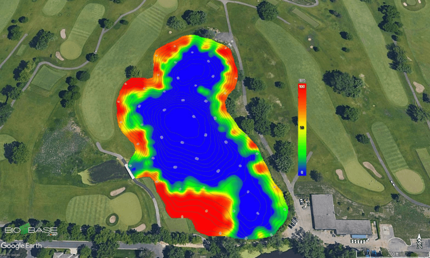
We recently began collection of baseline data on a small reservoir in northeast Washington State to gain a better understanding of the aquatic community and effects of the hydrological system on the flora and fauna. There is little public access and surveys along this stretch of river are limited. Flowering Rush and Eurasian Watermilfoil, both invasive plant species, have been identified in the reservoir, but distribution fluctuates coincident with changing water elevations and flows. Distribution of the plant community in the reservoir is not well understood. Traditional plant survey methods using the rake method are used to collect submerged plants, but the patches need to be located first. Bathymetric maps used previously were limited and we were looking for a good way to locate and map distribution of vegetation throughout the reservoir. Identification of the vegetation patches would allow us to target specific locations for invasive plant monitoring and inform fish surveys. To accomplish this, we used the Lowrance HDS12 with side and down scan capability. We made several tracks throughout the reservoir to maximize coverage and recorded all our movements on the Lowrance unit. The process was fairly simple…as we drove the boat around the reservoir, we recorded our tracks and saved the files as .sl3 files on the Lowrance unit, and uploaded them to the BioBase website. Once BioBase received the upload, they processed the data and we were then able to obtain bathymetric and vegetation heat maps that included vegetation percent biovolume such as the one shown below.
Since I was new to this product, I had a bit of a steep learning curve. [BioBase Product Expert] Ray Valley provided exceptional technical support in helping resolve challenges we faced during the initial setup and navigating the BioBase output. The outputs that we obtained from BioBase using the data (tracks) we recorded included bathymetry and aquatic distribution heat maps that provided a baseline for future invasive plant monitoring in this reservoir. Since we recorded several tracks, Biobase processed them individually which provides the user with the ability to look at smaller sections or to combine areas into a larger picture. The user should check the outputs to confirm the information provided in the outputs matches known site conditions. This information will be used to guide fish surveys and inform invasive species management in the reservoir. This product performed as promised by BioBase and met our expectations. We found this to be a valuable tool that we will continue to use for additional vegetative mapping and delineation to inform management of invasive species.
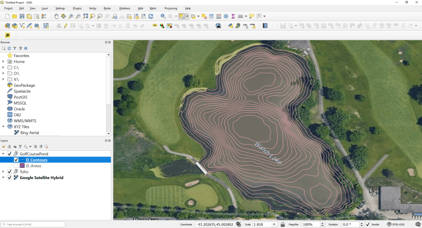
BioBase’s primary strength is its power as an automated processing engine delivering high quality geospatial data layers on aquatic habitats with very little user input outside of the physical effort to drive a boat and passively log sonar over an area of interest. In addition to the online analysis tools within BioBase like the polygon tool and automated statistical reports, users can export raw depth, vegetation, and bottom hardness data along their track, in X,Y,Z grid format, Google Earth imagery, Lowrance or Simrad Charts, AND NOW ESRI SHAPEFILES OF DEPTH CONTOURS! This feature has been in high demand for survey companies and governments who require detailed water volume analysis for aquatic habitat and fisheries management. Below we walk you through some helpful tips about the feature and how to use it.
Go To Tools – Export Data and click “Depth Shapefiles”
Example from a big lake:
D_Areas are polygon areas of each contour interval. Depending on your needs, you can calculate water volume by depth with the area of these “disks” or dissolve them to create a custom colored depth chart. D_Contours are contour polylines. NOTE: shapefile exports do not come with a projection and are in the WGS 84 global coordinate system (CRS 4326). If your GIS system doesn’t like you and says it can’t draw because there is no projection, select WGS84.
Example from a small pond:
5.8 acre (24,281 sq. m) pond as viewed in BioBaseExported 1ft contours. The user can control whether contours are in imperial or metric, but the values are always stored in metric (e.g., for the 1ft contour, the VALUE field in the attribute table will show 0.3048). For metric contours, they come out in 0.25m intervalsDepth Areas as polygons are also bundled into the zipped export. This will allow the user to carry out detailed water volume analysis as a function of depth with fewer post-processing steps than were originally required when data was only exportable as points. The VALUE field in the Attribute table is the Contour value in meters and VALUE2 is the outer range or deeper contour value of the Depth Area polygon.
BioBase continues its mission to deliver water and fisheries resource professionals high value data products in the hopes that you can focus less of your efforts on making maps and more on the important tasks of research and conservation.
2020 has been a busy year for BioBase improvements and new feature releases. Previously exclusive to BioBase’s sister consumer mapping platform, C-MAP Genesis, BioBase users can now export their bathymetric, aquatic vegetation heatmap, or bottom hardness map in a file format (AT5) that is compatible with most newer generation Lowrance and Simrad chartplotters. This feature enables researchers and aquatic resource managers to return to surveyed areas of interest and precisely target follow-up surveys or management actions (e.g., strategic taking of water or aquatic plant samples, placement of fish habitat structures or aeration equipment, precision applications of aquatic herbicides, etc.)
In the images and captions below, we’ll walk you through how to do this in your biobasemaps.com account.
Register your Lowrance or Simrad Chartplotter in your BioBase Account
Assuming you have already recorded your sonar data and successfully uploaded to biobasemaps.com, log into your BioBase account. Click “Plotters”Add unique details of your chartplotter. This feature is compatible with most newer (newer than 2014) Lowrance and Simrad GPS capable devices (e.g., Lowrance HDS, Elite Ti and Ti2, Simrad GO and Evo)Look in the “About” menu of your Chartplotter. Image above is from a Lowrance HDS Carbon.Look for the Serial Number and Content ID alphanumeric code. Enter these into the plotter form on biobasemaps.com
2. Export the GPS Chart file from the desired EcoSound Trip or Merge from BioBase.
In the Export Data tool, select “GPS Chart Generation”Export the desired layers
3. Unzip the downloaded file and save to a MicroSD card (<32 GB).
The layer will export as .zip with a random GUID name. The zip file must be unzipped (7-Zip is a great freeware for unzipping files) and the entire contents of the extracted zip file should be copied to a MicroSD card. The contents in the folder are propriety, encrypted files (.AT5) that are specific to the device you registered in your account. The chart file will not work in other non-registered devices. You can register multiple devices. One card can hold multiple AT5 folders (charts) and recorded sonar logs. Cards cannot be larger than 32 GB however.
4. View and Use in your Lowrance or Simrad!
Insert the card with the saved AT5 chart files. Go to the Chart and select the appropriate Chart Source in Chart Options. Voilà!Sample bottom hardness map from the same BioBase survey.If you want to view a blue- (or custom-) shaded contour map, simply uncheck the Vegetation/Composition categories in one of the Chart menus.Detailed, custom-made bathymetric chart. Note that prior to using for navigation, close attention by the user should be given to the quality of the sonar data recorded and resulting accuracy of the map.
At C-MAP, we are excited to announce the release of a new feature that allows users to export exact replicates of their BioBase EcoSound maps as Google Earth images (.kmz and .kml; Figure 1). This YouTube video will walk you through how it’s done.
Figure 1. Image of seagrass cover in Newport Bay, CA USA mapped with Lowrance, processed with BioBase EcoSound and exported as a Google Earth .kmz file. Example can be found in the free demo account on http://www.biobasemaps.com.
BioBase processed raw sonar logs and creates habitat maps with sophisticated algorithms. The outputs you see in BioBase are tiled georectified images (.png) of the outputs. The Google Earth feature converts the .png images to Google Earth’s .kml and .kmz file format. .kml downloads are smaller and reference the images on BioBase servers. .kmz downloads are larger and are exact copies of the images stored on our servers. The .kmz option is best for users who wish to archive local copies of their BioBase maps.
These images allow BioBase users to share spatial files with their stakeholders in a free Google format with which many are familiar and use regularly. Recipients can interact with the output zooming in and out to their desire and also adding custom logos and waypoints as they wish (Figure 2).
Figure 2. Add your own logos and other information to the Google Earth exported BioBase EcoSound image
Further, there are a range of open source tools that will convert .kml and .kmz to GIS files for use in ESRI and QGIS products. Given the popularity and widespread use of .kml and .kmz files, there are a range of other applications that we are eager to hear about. Please feel free to share in the comments below.
Converting EcoSound .kml/.kmz files to ESRI Layers (.lyr)
Special thank you to Kevin Johnson and Jennifer Moran at FL Fish and Wildlife Conservation Commission for sharing a tutorial about how to convert .kml/.kmz files to ESRI Layer (.lyr) files for analysis and overlays in ESRI GIS products:
Open ArcMap
Open ArcToolbox > Conversion Tools > From KML > KML to Layer
Input KML File
Toggle to saved .KML file Lake_Kerr_Biobase.kml (example) > Open
Output Location
Default output location is Documents\ArcGIS > Click the folder icon on right and toggle to appropriate folder
Output Data Name (Optional)
Will typically show the name of the kml, change if preferred
Select Checkbox for Include Ground Overlay (optional)
Only necessary for Raster data. Not necessary for lines/points/polygons
*This will take some time to process/load and will show up in ArcCatalog as “FileName.lyr”. Processing will depend on the file and image size. After it displays in the catalog, drag and drop or select Add Data to display the layer on the map.
**Arc GIS may shut down/disappear. You may not receive a green checkmark for execution completion. Reopen the program and go into your Catalog. Should not need to reconvert from .kml.
Lake Kerr (FL USA) aquatic vegetation heat map as seen in BioBaseLake Kerr (FL USA) aquatic vegetation heat map as seen in Google EarthLake Kerr (FL USA) aquatic vegetation heat map converted to a .lyr file in ArcGIS
Ok, it’s a bit overdue. But better late than never! BioBase customers will now see an updated and enhanced viewer for their EcoSound and EcoSat. No longer will users have to struggle to get their map to fit within the little square box of the old viewer with a Bing zoom level that either zoomed too close and cut off parts of the waterbody, or too far to see detail. Below we show you a few screenshots of the major improvements. You can see for yourself by logging into your own account or clicking the Log into DEMO button on the home page of biobasemaps.com, finding a waterbody of interest, and click on the Analyze/Edit button.