Lake Minnetonka is one of the largest and most heavily used recreational lakes in Minnesota and is composed of an interconnected system of bays (Figure 1). Every summer, a rooted invasive aquatic plant, Eurasian watermilfoil creates thick bottom to surface mats in many areas of the lake. While these mats may occur anywhere on the lake, they generally are thickest in certain shallow areas such as the Diamond Reef area in the main lake of Lake Minnetonka (officially described as Lower Lake North). This reef is popular with anglers, power boaters, and sailors. On any given night or weekend, well over a hundred keelboats may take part in regular club racing events or regattas here. World class level sailors, including Olympic champions, America’s Cup, and other accomplished sailors regularly race on the lake and the competition can be intense. When competition is tight, every advantage is important.
Figure 1. Lake Minnetonka; a popular recreational and fishing lake just west of the Twin City metropolitan area of Minnesota. The red box highlights an area popular with boaters, anglers, and sailors. The blue contoured areas represent areas uploaded and processed by anglers using the Genesis mapping service and aggregated into the C-MAP social map. Social maps can also be viewed in the C-MAP App.
2020 has been a busy year for BioBase improvements and new feature releases. Previously exclusive to BioBase’s sister consumer mapping platform, C-MAP Genesis, BioBase users can now export their bathymetric, aquatic vegetation heatmap, or bottom hardness map in a file format (AT5) that is compatible with most newer generation Lowrance and Simrad chartplotters. This feature enables researchers and aquatic resource managers to return to surveyed areas of interest and precisely target follow-up surveys or management actions (e.g., strategic taking of water or aquatic plant samples, placement of fish habitat structures or aeration equipment, precision applications of aquatic herbicides, etc.)
In the images and captions below, we’ll walk you through how to do this in your biobasemaps.com account.
1. Export the GPS Chart file from the desired EcoSound Trip or Merge from BioBase.
In the Export Data tool, select “GPS Chart Generation”Export the desired layers
3. Unzip the downloaded file and save to a MicroSD card (<32 GB).
The layer will export as .zip with a random GUID name. The zip file must be unzipped (7-Zip is a great freeware for unzipping files) and the entire contents of the extracted zip file should be copied to a MicroSD card. The contents in the folder are propriety, encrypted files (.AT5) that are specific to the device you registered in your account. The chart file will not work in other non-registered devices. You can register multiple devices. One card can hold multiple AT5 folders (charts) and recorded sonar logs. Cards cannot be larger than 32 GB however.
2. View and Use in your Lowrance or Simrad!
Insert the card with the saved AT5 chart files. Go to the Chart and select the appropriate Chart Source in Chart Options. Voilà!Sample bottom hardness map from the same BioBase survey.If you want to view a blue- (or custom-) shaded contour map, simply uncheck the Vegetation/Composition categories in one of the Chart menus.Detailed, custom-made bathymetric chart. Note that prior to using for navigation, close attention by the user should be given to the quality of the sonar data recorded and resulting accuracy of the map.
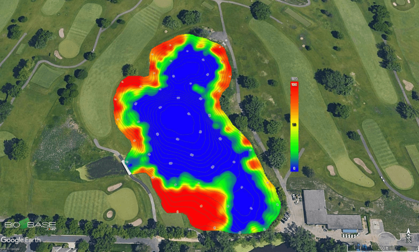
At C-MAP, we are excited to announce the release of a new feature that allows users to export exact replicates of their BioBase EcoSound maps as Google Earth images (.kmz and .kml; Figure 1). This YouTube video will walk you through how it’s done.
Figure 1. Image of seagrass cover in Newport Bay, CA USA mapped with Lowrance, processed with BioBase EcoSound and exported as a Google Earth .kmz file. Example can be found in the free demo account on http://www.biobasemaps.com.
BioBase processed raw sonar logs and creates habitat maps with sophisticated algorithms. The outputs you see in BioBase are tiled georectified images (.png) of the outputs. The Google Earth feature converts the .png images to Google Earth’s .kml and .kmz file format. .kml downloads are smaller and reference the images on BioBase servers. .kmz downloads are larger and are exact copies of the images stored on our servers. The .kmz option is best for users who wish to archive local copies of their BioBase maps.
These images allow BioBase users to share spatial files with their stakeholders in a free Google format with which many are familiar and use regularly. Recipients can interact with the output zooming in and out to their desire and also adding custom logos and waypoints as they wish (Figure 2).
Figure 2. Add your own logos and other information to the Google Earth exported BioBase EcoSound image
Further, there are a range of open source tools that will convert .kml and .kmz to GIS files for use in ESRI and QGIS products. Given the popularity and widespread use of .kml and .kmz files, there are a range of other applications that we are eager to hear about. Please feel free to share in the comments below.
Converting EcoSound .kml/.kmz files to ESRI Layers (.lyr)
Special thank you to Kevin Johnson and Jennifer Moran at FL Fish and Wildlife Conservation Commission for sharing a tutorial about how to convert .kml/.kmz files to ESRI Layer (.lyr) files for analysis and overlays in ESRI GIS products:
Open ArcMap
Open ArcToolbox > Conversion Tools > From KML > KML to Layer
Input KML File
Toggle to saved .KML file Lake_Kerr_Biobase.kml (example) > Open
Output Location
Default output location is Documents\ArcGIS > Click the folder icon on right and toggle to appropriate folder
Output Data Name (Optional)
Will typically show the name of the kml, change if preferred
Select Checkbox for Include Ground Overlay (optional)
Only necessary for Raster data. Not necessary for lines/points/polygons
*This will take some time to process/load and will show up in ArcCatalog as “FileName.lyr”. Processing will depend on the file and image size. After it displays in the catalog, drag and drop or select Add Data to display the layer on the map.
**Arc GIS may shut down/disappear. You may not receive a green checkmark for execution completion. Reopen the program and go into your Catalog. Should not need to reconvert from .kml.
Lake Kerr (FL USA) aquatic vegetation heat map as seen in BioBaseLake Kerr (FL USA) aquatic vegetation heat map as seen in Google EarthLake Kerr (FL USA) aquatic vegetation heat map converted to a .lyr file in ArcGIS