
What is EcoSat?
EcoSat delivers a one-of-it’s-kind semi-automated cloud processing of very high resolution satellite imagery to map nearshore vegetation and coastal benthic habitats. EcoSat uses the latest multi-spectral imagery from reputable providers such as Digital Globe (World View 2,3 and 4), Airbus Defence and Space (Pleiades), and ESA’s Sentinel program and industry standard image processing techniques. Sophisticated Amazon Web Service cloud infrastructure rapidly processes imagery, creates reports and imagery tiles, and delivers detailed habitat maps to user’s BioBase dashboard where it can be analyzed and shared. Average turnaround time from imagery tasking order to delivery of results is 60 days. The rapid and standard processing methods are allowing entities like the Florida Fish and Wildlife Conservation Commission to establish regular monitoring programs for emergent vegetation. The extremely long and expensive one-off nature of conventional remote sensing mapping projects using non-repeatable tailored techniques has prevented natural resource entities from assessing the degree that habitats are changing as a result of environmental stressors such as invasive species invasions and climate change.
Can EcoSat Identify Vegetation Species?
Yes! Using the industry-standard Random Forest method of machine learning, EcoSat can employ supervised classification methods using training data from users, or unsupervised classification based on automated pixel/object clustering. Supervised classifications produce actual vegetation species classifications as seen in Figure 1. If no training data exist or species communities are mixed, unnamed objects are delineated and the user can go in later and add names to classifications or group classes as they see fit (Figure 2).


How do I Know Vegetation Classifications Are Accurate?
In large part, this is up to you. If you have greater than 15 in situ points (the more the better) collected from the interior of large monotypic beds, then the machine learning process will know to correlate a particular spectral response to your input information. See the images below that will help you to create robust classifications.


A second way to verify classifications is to take your map out into the field. We make the validation process easy by giving you waypoint creation tools in EcoSat and also automatically generate a Lowrance or Simrad GPS chart of classifications that you can take out into the field with you (Figure 6).

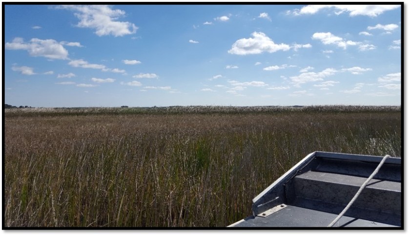
What I see from my boat doesn’t match what EcoSat tells me. Why?
The answer to this question partially lies within the concept of Minimum Mapping Unit (MMU). The MMU is the smallest scale at which an object is mapped as a discrete entity. Any object smaller than the MMU is incorporated into a larger object within which it is nested. At the smallest scale, the image resolution (e.g., pixel size) could be the MMU. However, images from large scenes quickly get overwhelmingly busy with detail (Figure 7). As such, it is common to use a larger MMU to create more generalized maps of natural features.

A problem occurs however when the biologist ventures into the field and navigates to a random validation waypoint and happens to land within a vegetation bed that is either less than the MMU or their field of view is greater than the MMU. In both cases, what they write down in their field sheet will not correspond to what is classified by EcoSat (Figure 8). As such, it is important that the scale of field verifications match the scale at which vegetation “objects” are being classified in EcoSat. Or, collect several verification points within an aggregated bed

Digging deeper into supposed misclassifications – GPS error:
Figure 9 demonstrates another issue where a spreadsheet may indicate misclassifications but a closer look in GIS would indicate measurement error as the cause. In this example, the field biologist captured a verification waypoint on the edge of a maidencane bed next to a bulrush bed. Consumer GPS typically has a 2m deviation in any one direction for spot locations. A straight-up spatial join in GIS shows that the satellite classification wrongly classified maidencane as bulrush. But a closer look in GIS suggests the classifications was actually correct. Lesson learned: ensure GPS calibration and verification waypoints are captured in the middle of homogenous beds.

Harness the power of the cloud to iteratively learn and rapidly map vegetation and coastal habitats
As more processing rules are established and species classification libraries grow (not to mention steady increases in computing power and sensor resolution), outputs will be even more precise and accurate, faster, and cheaper. This will empower natural resource managers with more and better information about the status of natural habitats and facilitate more effective conservation.
![]()